
Appendix C - Interpolation
Interpolation consists of generating data points between given coordinate axis positions and using this data to generate a path in space (linear, arc, circle, or helix) related to the coordinated axes.
With linear interpolation, these points establish a straight-line path through space of the associated axes. With Commander, an interpolation causes the axes to move simultaneously from the start to the end of the command. The interpolation calculates individual axis velocities to drive the axes along the desired path at the given feed rate. Thousands of intermediate coordinate points along the path are calculated between the start point and the end point of the move.
Commander series of controllers utilizes linear interpolation (linear coordinated motion between two to four axes), arc and circular Interpolation with any two axes, and helical Interpolation with X, Y and Z axes (arc and circle (X, Y) in combination with linear interpolation (Z-axis)). Interpolation operation can be executed up to the maximum pulse frequency.
In this section
- Linear Interpolation
- Arc Interpolation
- Circular Interpolation
- Helical or Tangential interpolation (Circular Interpolation Synchronized with the U-axis)
- Additional notes regarding Interpolation functions
C.1 Linear Interpolation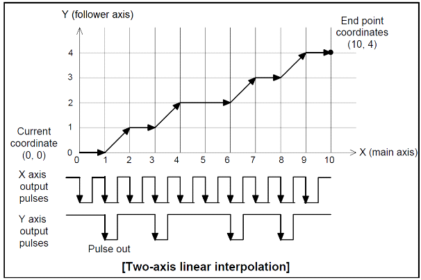
To execute a linear interpolated move, specify the endpoint coordinates and the desired linear interpolation operation. The endpoint is specified as an incremental number of pulses from the current position on each axis, or the desired absolute position coordinates. Commander automatically identifies the axis with the larger feed distance as the main axis, and the other axes as the secondary axes. The main axis is supplied a pulse rate tied to the specified feed rate, while the secondary axes are supplied with a reduced pulse rate based on the interpolation calculations.
Precision of linear interpolation
As shown in the figure on the right, linear interpolation executes an interpolation from the current coordinates to the end coordinates provided. The positional precision of a specified line during linear interpolation will be ±0.5 LSB throughout the interpolation range.
"LSB" refers to the minimum feed unit for the system. It corresponds to the resolution of the mechanical system. (Size of the cells in the figure on the right.)
See the PCL6045BL manual, section 9.8.5 for more information.
C.2 Arc Interpolation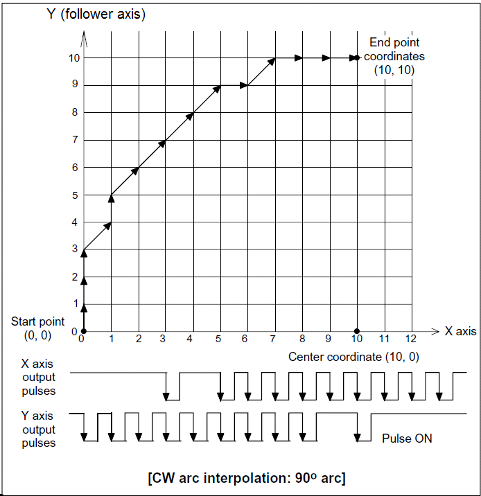
Executing an arc interpolation from the current position as the starting point requires the center coordinates and endpoint of the arc in degrees. Select either a CW or CCW arc interpolation direction and enter the arc center coordinates (incremental or absolute) and arc travel endpoint in degrees. The CW arc interpolation draws an arc from the current coordinates to the endpoint coordinates in a clockwise direction, using the center coordinates as the arc center. The CCW arc interpolation draws an arc in a counterclockwise direction.
The figure to the right is an example of drawing an arc with the X and Y axes in a CW arc interpolation operation
See the PCL6045BL manual section 9.8.8 for more information.
C.3 Circular Interpolation
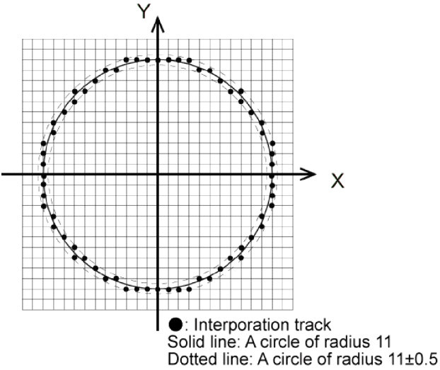
Executing circular interpolation from the current position as the starting point requires the center coordinates of the circle. Select either a CW or CCW circular interpolation direction and enter the circle center coordinates (incremental or absolute). The circular interpolation function draws a circle from the current position to the end coordinate, moving CW or CCW. The positional deviation from the specified curve is ±0.5 LSB. The LSB corresponds to the resolution of the mechanical system (size of the cells in the figure).
The figure on the right is an example of how a simple circle with a radius of 11 units is created.
C.4 Helical or Tangential interpolation (Circular Interpolation Synchronized with the U-axis)
The Commander series of controllers allows a combination of circular or arc interpolation of X and Y axes with linear interpolation of the Z-axis to provide a helical path of motion. The U axis is used in the background as a virtual axis to aid in the performance of this function. This feature is used in applications that may require circular interpolation between the X and Y axes, and to adjust the angle of a jig toward an arc tangent point with the Z axis. Since the U axis plays a role in these moves, it cannot be used for any other purposes.

C.5 Additional notes regarding Interpolation functions
Acceleration/deceleration operations
Acceleration and deceleration (linear and S-curve) can be used with linear, arc, and circular interpolation operations.
Error stop
If any of the axes performing interpolated movements stops with an error, all of the axes performing interpolation will stop.
SD input
When SD input is enabled and turns ON for any axis during an interpolation operation, all axes will decelerate or decelerate and stop.
Idling control
If any axis is in idling range, none of the axes performing interpolation will accelerate.
Correction function
When a direction is changed by switching of quadrants during circular interpolation, backlash correction and slip correction control cannot be used.